Using scikit-learn to create a model

Getting started #

Scikit-learn is a set of tools for creating machine learning models. Or in their words a "Simple and efficient tools for predictive data analysis".

Their installation guide got me going. The creation of a Python virtual environment is recommended, to isolate project work from the verison of python installated on the machine. Assuming Python3:

python -m venv sklearn-env
source sklearn-env/bin/activate
pip install -U scikit-learn

But I didn't find their guides all that helpful to get going after that. I know I wanted to use Jupyter. Here are the steps I found to set up everything else needed. The ipykernel adds the ability to create a new Jupyter notebook kernel which will contain all of the installation bits for the python virtual environment being used.

pip install jupyterlab
pip install ipykernel
python -m ipykernel install --user --name scikit-kernel
pip install matplotlib numpy pandas seaborn

Start up with jupyter lab and we're off and running. Create a new notebook using the scikit-kernel we just created.

Now what? I didn't find the documentation particularly helpful, so off to YouTube! I found this freeCodeCamp.org video helpful, Scikit-learn Crash Course - Machine Learning Library for Python, at least the first few modules. The rest of this post will be based upon what I learned in this video.

The data #

The course uses the Boston house price dataset. This dataset has been removed from scikit-learn, as explained in the video. If you want to follow along with the tutorial you either need to install an older version of scikit-learn, or I found you can still access and load the data with this script:

import pandas as pd
import numpy as np

data_url = "http://lib.stat.cmu.edu/datasets/boston"
raw_df = pd.read_csv(data_url, sep="\\s+", skiprows=22, header=None)
X = np.hstack([raw_df.values[::2, :], raw_df.values[1::2, :2]])
y = raw_df.values[1::2, 2]

While watching the video I did use the Boston dataset. After completing the video I went back and reran the example using the California housing dataset, which is included in scikit-learn:

from sklearn.datasets import fetch_california_housing
california_housing = fetch_california_housing()
X, y = california_housing.data, california_housing.target

But I wanted to apply what I learned to a real dataset. Therefore, at my job I created a SQL script to extract data from a database for a business scenario I thought it would be interesting to make predictions for. The dataset has approximately 100k records. I'm using this data for the rest of the blog post. Since it is real data I'm not revealing any of the data. I have also removed columns which do not add any value to the blog post and I have changed some of the column names.

Loading things up #

In the first notebook cell I import everything I'll eventually use. Therefore, I won't explain any of it here.

import matplotlib.pylab as plt
import pandas as pd

from sklearn.neighbors import KNeighborsRegressor
from sklearn.ensemble import RandomForestRegressor

from sklearn.preprocessing import StandardScaler, OneHotEncoder
from sklearn.pipeline import Pipeline
from sklearn.model_selection import GridSearchCV

Pandas, commonly abbreviated pd has a lot of functionality for working with data. It has a handy function to read in data from a CSV into a DataFrame, the default tabular structure for holding the data.

orig_data = pd.read_csv("sample.csv")

Categorical data #

The dataset has both numerical and categorical data. Additionally, some of the categorical data it makes sense to group together into buckets. For this example, I have a column named "class" which has positive integer values. Each value represents a particular class and each 100 value range represents a kind of class. Therefore the data can be segmented into 100 value groups.

To do this the Panada's cut function can be used, to target one column and group each value into a group, i.e. "bin". We therefore create an array of "bins" to define the grouping, as well as labels, which will be the new column names. Once the new columns have been created for each group we can remove the original "class" column:

class_bins = [0, 99, 199, 299, 399, 499, 599, 699, 799, 899, 999, float('inf')]
class_labels = ['0-99', '100-199', '200-299', '300-399', '400-499', '500-599', '600-699', '700-799', '800-899', '900-999', '1000+']

orig_data['class_ranges'] = pd.cut(orig_data['class'], bins=class_bins, labels=class_labels, right=True)
data_with_ranges = orig_data.drop(['class'], axis=1)

All categorical columns now need to be encoded. They need to be transformed so that the model can create relations between the categorical values. Each column to encode is specified, transformed into an encoded array, placed into a DataFrame along with their column names and then included into the original dataset. Finally the original columns are removed:

catgorical_encoder = OneHotEncoder(sparse_output=False)
catgorical_columns = ['gender', 'marital_status', 'class_ranges']
encoded_array = catgorical_encoder.fit_transform(data_with_ranges[catgorical_columns])

encoded_data = pd.DataFrame(encoded_array, columns=catgorical_encoder.get_feature_names_out(catgorical_columns))
data = pd.concat([data_with_ranges, encoded_data], axis=1).drop(catgorical_columns, axis=1)

We have "preprocessed" our data. We now can break our data up into "features" and a "target", or commonly referred to "X" and "y". The features are what we are using to make predictions. The target is the real value we are desiring to predict. This is "supervised" learning. In our date the target is the column "late", indicating whether the item is either late or not, 0 or 1.

X = data.drop(['late'], axis=1)
y = data['late']

The pipeline #

Once we have our data we can immediately send it to a model for training and prediction. But typically a more elaborate "pipeline" is used, which can be thought as a model itself, to make further tweaks to the data.

The first piece of our pipeline is to scale the values in our data. If some columns have values which range from 1-10 but other columns 1-1,000,000, then the significance of the values in the first column will be lost. Therefore, all numerical values are scaled so that some do not overpower others.

The second piece of the pipeline is what model to use. We will start out with the K Nearest Neighbors model. I will not try to describe how any of the models work, that is an immense topic. I encourage you to use your favorite search tool to find an article which provides you a helpful description.

Here is our pipeline:

pipe = Pipeline([
    ("scale", StandardScaler()),
    ("model", KNeighborsRegressor())
])

We could train and predict using this pipeline, but we have a couple more concerns to consider.

First, each model has parameters which can be tweaked. You can see the names of these parameters by calling pipe.get_params(). For the nearest neighbors model a property of interest is how many neighbors to use, "model__n_neighbors". The default value is 5, but what value is best for our data?

Second, our predictions will be biased if we use the same data for training as we do to make predictions. Therefore, the data should be split up into a set for training and a set to make predictions. How the data is split can also influence the result of our model. Therefore, it would be even better if we can split of the data, train and then split up the data another way and train again with that version of the split data.

We can accomplish both of these things using a grid search cross validation. Below, we specify how many times to split up the data cv=3 and which model parameters to target and the values to use param_grid={'model__n_neighbors': [3, 5, 7, 9]}. This will create 9 training sets, a combination for each value.

model = GridSearchCV(estimator=pipe,
             param_grid={'model__n_neighbors': [3, 5, 7, 9]},
             cv=3)
model.fit(X, y)

We can see the results of the grid search by calling pd.DataFrame(model.cv_results_). This will show how each combination preformed and will rank them. For the dataset I'm using none of the combinations performed well. Nevertheless, for now we'll continue on making predictions, which is as simple as prediction = model.predict(X).

Visualizing the results #

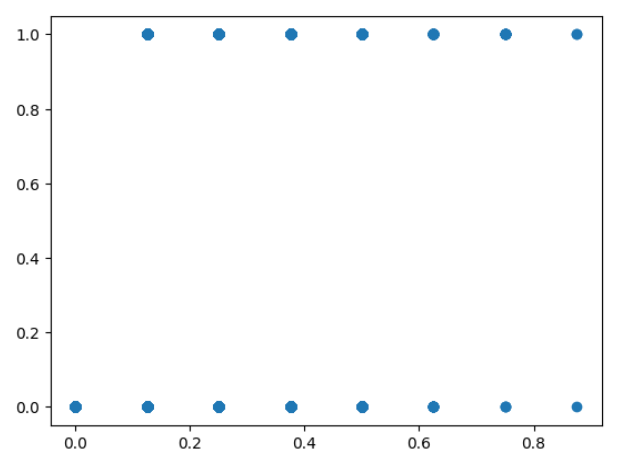
The predictions can be visualized with a scatter plot, plt.scatter(prediction, y). Unsuprisingly, the predictions do not make sense, they jump all over the place.

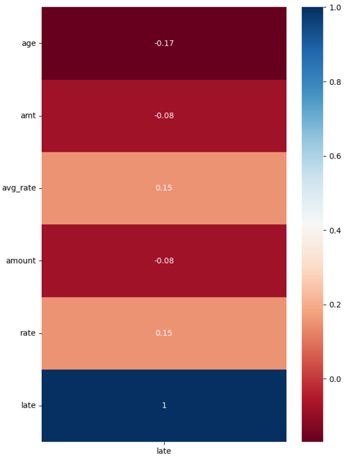
A heatmap can also be displayed showing the correlation of each feature to the predicted target. For our data there is not any features strongly correlated.

import seaborn as sns
from matplotlib.patches import Rectangle

heatmap_data = X
heatmap_data['late'] = prediction

fig, ax = plt.subplots(figsize=(7,20))
sns.heatmap(heatmap_data.corr().iloc[-1,:].values.reshape(-1,1).round(2), annot=True, cmap='RdBu')
ax.set_yticklabels(heatmap_data.columns.tolist(), rotation=0)
ax.set_xticklabels(['late'])

What next #

In this particular case the results obviously do not make sense. It clearly indicates we need to either use other data, reconsider how we are preprocessing the data we have, try other models or try other parameters with our current data.

I went down the route of using several other models. One model which produced results which seem to make sense is the RandomForestRegressor. Here's are new pipeline:

pipe = Pipeline([
    ("scale", StandardScaler()),
    ("model", RandomForestRegressor())
])

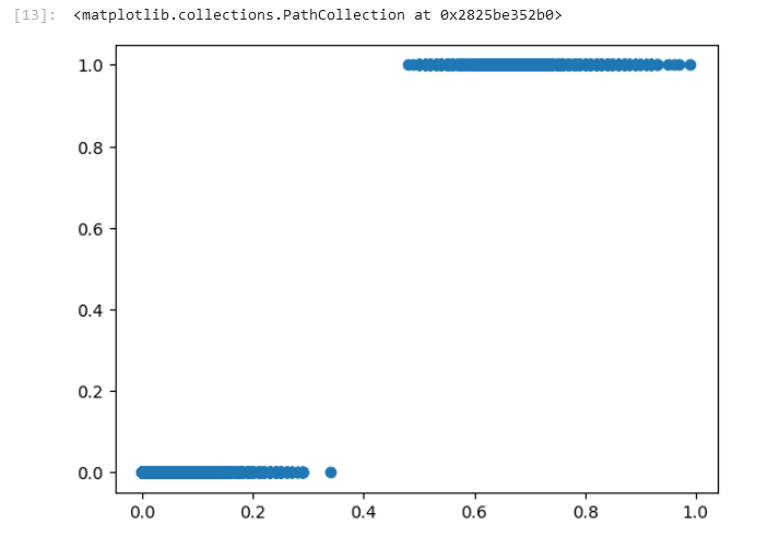
We can then use the grid search and make a prediction again. Here's the new plot:

These results make much more sense. When it predicts values less than .4 it seems to indicate the correct target of not "late". When above .4 then it is "late".

Conclusion #

We are not finished yet. We have a result, but can the result be trusted? It seems a little too good. Is it overfitted to our data?

We are just getting started. We've done the easy part, creating a functional model. Now we need to apply our understanding to evaluate what's going on.